Week 10: GIS Applications

From August 29 to September 2, 2009, one of the largest fires the Los Angeles County has seen in years claimed the lives of two firefighters, burned more than 100,000 acres and 80 residences, and in total threatened more than 12,500 homes (CNN, L.A. Times, KABC). While the 2009 Station Fire originated from a sudden, unpredictable and unnatural cause — the arsonist was never found, according to KABC — the fire was likely so severe and so wide in its scope because natural and human-made conditions were setting the stage for such a destructive fire. In this report I will use GIS overlay analysis and draw upon scientific literature to see what might have led to the immense severity of this fire and what we can do to minimize damage done to the area in future fires.

Here is a reference map showing the Los Angeles County and the perimeters of the Station Fire as it spread over time. The map also shows the boundaries of the areas that each Los Angeles County fire station is responsible for protecting in the case of a fire.

Here is a map of past fires preceding the Station Fire from 2000-2009 and also of the Los Angeles National Forest, which is shaded in green. Although the National Forest indeed only comprises the political boundaries of just one certain ecosystem or fuel source, because the 2009 Station Fire burned almost entirely within the confines of the National Forest, I believe it was suitable to analyze the fuel history of that forest to see what might have led to such a big Station Fire. As we can see in this map, fuel has been allowed to accumulate in the Los Angeles National Forest area in the years leading up to the Station Fire. The Los Angeles National Forest has not seen any significant fires really since 2002, and those fires covered at most just half the area that the Station Fire did. More importantly, almost no fires burned in the Station Fire area in the nine years leading up to the Fire, signaling that this area likely accumulated forest debris and, subsequently, the fuel to supply a disastrous fire like the one that occurred in 2009.

It is also interesting to note that the greatest number of fire stations are in the southeast part of the Los Angeles County, a huge part of the county that has not seen any large fires in ten years. This seems to support the idea that fire suppression efforts are concentrated especially in areas where there are large numbers of population, a phenomenon I will examine further in this report.

An example of fire suppression: using chemical fire retardants to halt the advance of fire. Source: Times of Israel.

One issue connected to this problem of fuel buildup is that of fire suppression. While we must obviously try to protect civilians and their property from being destroyed by any fire, fire suppression over time can have negative effects on Southern California's ecosystems and can even lead to worse future fires. This is because fires are crucial for maintaining Southern California's Mediterranean ecosystems. Southern California's naturally dry chaparral and other shrubs are adapted to fire and depend on low amounts of it to destroy old matter and make way for new growth. Otherwise, dead debris from these plants accumulate and lead to "a gradual increase in dead fuels... (which) is a major cause of increasing flammability" (Conard and Weise). Fire suppression not only involves technology that can be very harmful to the environment, such as tractors, explosives and chemical retardants, but it can contribute to this buildup of fuel by preventing fires from gradually clearing it over time (National Wildlife Coordinating Group, Backer, Jensen and McPherson).

The rest of this report attempts to explain the apparent trend between fire suppression efforts and the location of civilian populations.

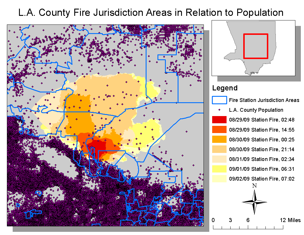
Here is a map showing the relation between population and fire station boundaries. This map supports my hypothesis that fire station boundaries — and thus the distribution of fire suppression efforts — are set with resident populations as one of the main priorities. Right below the Station Fire perimeter is an extremely dense band of residents, and this band also coincides with a band of many fire station areas. Thus this map shows that the allocation of fire suppression efforts are determined primarily according to population.

This map shows how resident populations are distributed in the Station Fire area. From the map we can see that many people live right on the edge of the area where the Station Fire occurred, and even in the space that was consumed by the fire. It is important to note that the fire occurred almost entirely within the perimeter of the Los Angeles National Forest, and thus the Station Fire got all of its fuel from that forest. This creates an inherent problem for the people living in the Los Angeles National Forest area and also for the people living right on the border of the forest, since they were all in direct proximity to the Station Fire. Fire suppression efforts were understandably heavily directed towards protecting this border population, but repeated intense fire suppression leads to more fuel buildup and sets the stage for larger fires.

Therefore, because there are significant numbers of people living in this area where fuel buildup is most likely to occur due to the large number of trees and general biomass, it creates a recurring problem of fire suppression and fuel buildup. Fire suppression is likely to be more intense in these areas, preventing the forest from being cleared of debris that can intensify a wildfire.

Thus, after analyzing these maps, one can conclude that populations should be discouraged — and possibly even regulated — from living in or near the Los Angeles National Forest area and other areas where there are abundant fuel sources for fires. Having populations there will only lead to more fire suppression, more fuel buildup and more difficult fires for firefighters to deal with. If populations are relocated from that area, then small to moderate fires could be allowed to burn the fuel buildup there and thus create a healthier environment for both plants and people. There would also be a smaller need for more intense fire suppression, since people would be less immediately in danger of being touched by the fires.

Data sources

Los Angeles County enterprise GIS. http://egis3.lacounty.gov/eGIS/tag/shapefiles/.

UCLA's spatial data repository. http://gis.ats.ucla.edu//Mapshare/Default.cfm#.

Bibiliography

Backer, Dana, Sara Jensen and Guy McPherson. “Impacts of fire-suppression activities on natural communities.” Conservation Biology 18, No. 4 (2004): 937-945. Accessed March 18, 2013.

“'Angry fire' roars across 100,000 California acres.” CNN, August 31, 2009.  http://articles.cnn.com/2009-08-31/us/california.wildfires_1_mike-dietrich-firefighters-safety-incident-commander?_s=PM:US.

Conard, Susan and David Weise. “Management of fire regime, fuels, and fire effects in southern California chaparral: Lessons from the past and thoughts for the future.” National Agricultural Library: 342-350. Accessed March 18, 2013.

Friedman, Ron. “Firefighters gain control over Carmel blaze.” The Times of Israel, March 8, 2013. Accessed March 19, 2013. http://www.timesofisrael.com/firefighters-gain-control-over-carmel-blaze/.

Garrison, Jessica, Alexandra Zavis and Joe Mozingo. “Station fire claims 18 homes and two firefighters.” Los Angeles Times, August 31, 2009. Accessed March 18, 2013. http://articles.latimes.com/2009/aug/31/local/me-fire31.

Hernandez, Miriam. “Thursday marks Station Fire 1-year anniversary.” KABC, August 26, 2010. Accessed March 18, 2013.

Wildland Fire Suppression Tactics Reference Guide (National Wildfire Coordinating Group, 1996).

Week 9: Cartography

For this week, I created three maps based on data from the 2000 U.S. census.

Here is a map showing the Asian population percentages for each county. Unfortunately, with all three of my maps, some county polygons failed to calculate properly when I used the GIS calculator to find the population percentages. So, on all three of my maps, there are certain polygons that are left white and blank because the calculations did not go through. I was unable to fix the problem in GIS or locate the attributes that were not calculating properly. Out of all the three maps I made for this lab, it appears on this map that the Asian population seems to have the most varied locations where its population percentage is greatest. While the most concentrated Asian populations are on the west coast in California, some higher percentages are also scattered in various spots on both coasts, and some are scattered in the midwest.

Here is a map showing the black population in the U.S. It is obvious that the population is more concentrated in the South: out of all the three maps I made, this map has the clearest trend. I like how the color scheme worked out for this map's symbology: using a color scale that uses light shades to denote smaller percentages to heavy or bright shades of red for the larger percentages helps viewers more clearly see the large concentrations of the black population in the South.

Here is a map of other population percentages, namely populations that are not any of the U.S.'s major racial or ethnic groups, such as the Caucasian, black or Asian populations. I tried a new kind of  color scheme for the symbology on this map: this time, the darker blue colors indicate a higher percentage, while anywhere that is green will have low percentages from 0 to 2.31 percent. I thought this two-color scheme was appropriate to use for this map, since the range percentages that the green color represents are all pretty much the same, because they are so small. Thus it would not be a poor choice to use one color shade to represent these multiple percentage ranges. This color scheme allows the viewer to see more starkly and clearly where the variation in racial groups are, which are mostly in California and in the southwest. Also, the darker blue shades help denote where the diversity is even greater in these areas. However, I can see how this color scheme could lead to pitfalls, since it might lead the map viewer to make generalized assumptions about the area covered only by the same shade of green.

Considering the actual data involved in the making of these three maps, I'd say the third map of the "other" racial population percentages surprised me the most. I did expect the most diversity in California, but I did not expect as much diversity in Texas, New Mexico and even Colorado. It was unfortunate that a handful of counties were unable to be calculated in each map. But after completing three other exercises using GIS, these maps were not difficult for me to create. The only way I think these maps could be misleading is the fact that some counties are larger than others. Thus, the larger counties that take up more space on the map lead to a greater generalization of that area, while the other smaller counties are more accurate because they attribute a statistic to a smaller area. There could be any amount of variation within the larger counties that are masked because the entire county is covered by one color.

I have more respect for GIS than I did when I first started this course. I used to think it was too difficult for any common, non-GIS-trained person to use, but now I see that as long as somebody gets an initial introduction to how to use ArcMap, they can easily start making maps on their own. It especially helps that, when you place your cursor over each command button in ArcMap, it gives you a description of what that command does. I do wish I knew if ArcMap had more spatial analysis capabilities, since the only ones we had time to learn about in lab were overlay analysis and some raster analysis functions. But overall, GIS is very helpful in going beyond the capabilities of traditional print maps to portray information. It is much more flexible and allows the user to manipulate data using different geographic coordinate systems with precision, helping to eliminate the chance of human error. GIS is in some ways limited, however, whenever there are errors or glitches in the ArcMap program.